Monarch populations during the Dust Bowl years

Introduction

The concern about the potential listing of monarchs as threatened or endangered by the Fish and Wildlife Service sometime in 2024 has led me to look into the conditions prior to 1994-1996. The populations in those years were quite large, and it has been widely assumed that the numbers of hectares measured in Mexico represented what could be expected from year to year. I’ve been skeptical, and in a previous post, I summarized data for 15 years with 1 to 3 temperature or precipitation metrics that exceeded anything that occurred in the last 29 years. The data for these 15 years suggested that significant declines were likely in all but two cases. Two of those 15 years were in the 1930s – the “Dust Bowl” or what is sometimes referred to as the “Dirty Thirties”. This led me to ask how monarchs might have fared throughout this period.

If you haven’t read about the Dust bowl or viewed the Ken Burns dust bowl documentary, I highly recommend them. The stories and lessons are compelling and sobering (Egan, 2006). Sobering because we may be headed for more of the same in the future. Farming recovered rapidly in this region after WWII as farmers tapped into the Ogallala Aquifer. This aquifer consists of Pleistocene (fossil) water stored beneath the surface of an enormous area that extends from South Dakota well into the former dust bowl areas further south. Unfortunately, water is being withdrawn from the aquifer faster than it is being replenished with the result that wells are being abandoned in many areas, taking the region back to dryland farming and the conditions that led to the dust bowl. Further, increasing temperatures and severe drought are predicted for Texas and parts of the Midwest in the years to come (Nielsen-Gammon 2021). I will leave it for you, the reader, to educate yourself about the origins and broad consequences of this disastrous yet formative time in our history. My task is to bring together three things: 1) the geography of the dust bowl, 2) the areas from which most monarchs originate that reach Mexico and 3) the broad sweep of the weather that would have affected monarchs during this interval.

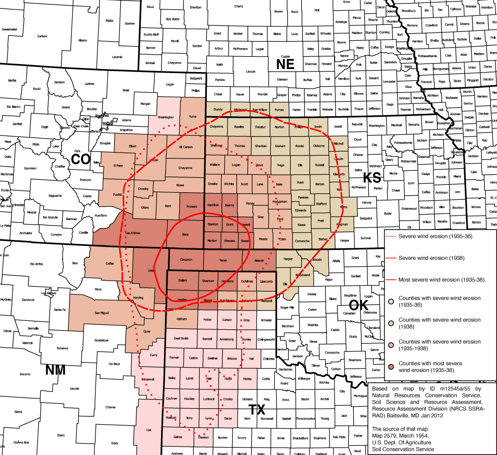
The dust bowl area, which is described as the High Plains or the southwestern Great Plains, encompassed portions of 6 states (Fig.1). Much of the dust bowl was bounded by 35N-40N latitude and 100W-105W longitude. The dust storms that characterized the region in the 1930s followed the conversion of the short grass prairies to wheat production and grazing in the early decades of the 20th century. The bare soils associated with farming, droughts and high winds led to dust storms that darkened the skies and spread dust as far as the east coast.

Figure 1. Dust bowl region showing areas and years of major dust storms. See “Dust Bowl” Wikipedia entry for more detail.

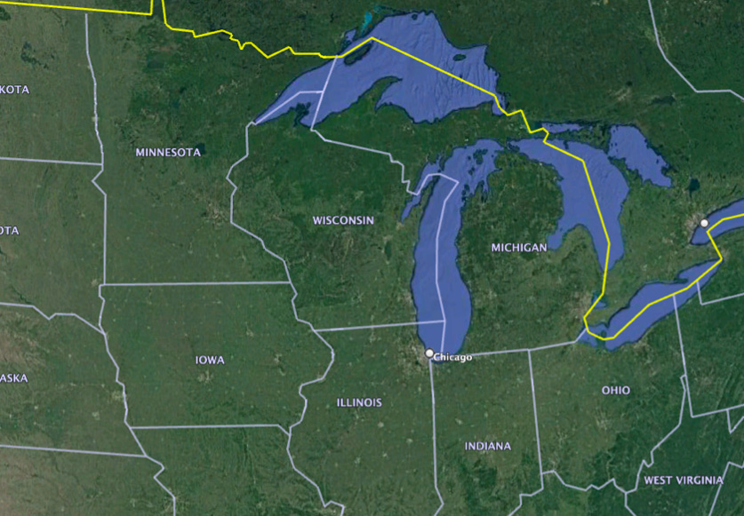
Short grass prairies are not major monarch production areas. Milkweeds are few, and nectar sources can be scattered and scarce for butterflies for parts of the breeding season. Further, the area is south and west of the major regions, Upper Midwest and Ohio Valley, that produce most of the monarchs that reach the overwintering sites in Mexico (Fig 2.) (Taylor, et al., in prep). So, if the region of the dust bowl is not a major production area, why is it of concern? Because what happened in the dust bowl from 1930-1939 occurred throughout the area east of the Rocky Mountains. These were the hottest consecutive 10 years during the growing season seen in the entire record from 1895-2022. This period was characterized by droughts, extreme low temperatures in the spring and higher than average summer temperatures in every year, except 1935, in that span. These conditions resulted in lower crop production in many areas to the east of the dust bowl region. And the dust itself settled widely with unknown consequences for foliage feeding insects and other herbivores.

In the following text, I’m going summarize how the growth of monarch populations was probably affected during this period. We now have a base of 29 years for which the conditions have been defined during the growing season. How these conditions affected the growth of monarch populations is now fairly clear. Average temperatures favor population growth while extreme temperatures, either above or below the long-term averages negatively affect population development. The negative factors have greater effects in March and April at the start of the growing season and lesser impacts in the summer and during the migration. Droughts that occur during the growing season or the migration can also limit population growth or the proportions of the population that survive the migration.

Methods

A series of metrics were chosen that represented critical times and locations associated with different stages in the development of the monarch populations. The long-term means and the deviations from these means are summarized in Table 1. These deviations were judged to be either favorable, neutral or unfavorable based on the assumption that there is an average range that enables population growth outside of which high or low temperatures were unfavorable. There are also a few conditions when high temperatures that occur when means are typically low are favorable. For temperature, the range for “average” conditions is >-3.3 – +2.5F. In other words, temperatures less than -3.3F and more than 2.5F were deemed as having a negative impact on population growth.

Table 1. Highest and lowest deviations from long-term means in the last 29 years.

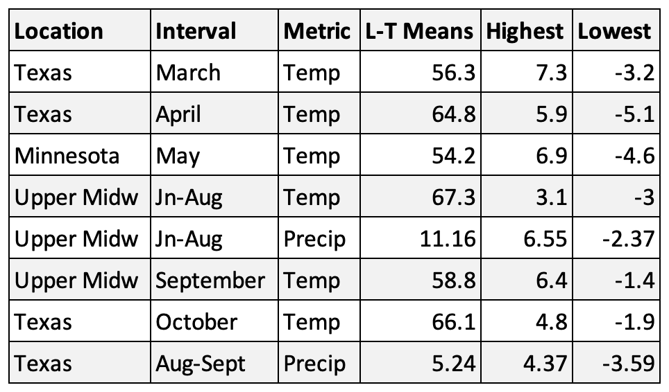
The effects of the deviations from long-term means for precipitation are more difficult to assess. Obviously, there can be too much precipitation, but there is no scale for too much rain. Furthermore, excessive rain tends to be local. In this case, I let the outcomes define the unfavorable conditions since there were years in which deficits of rainfall of as low as -2inches were associated with declines.

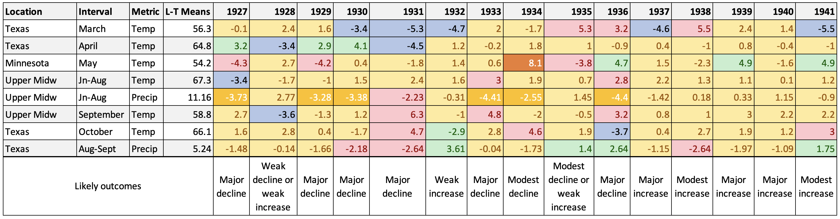
These criteria were applied to the deviations for 1927-1942 in Table 2. I added years on either side of the dust bowl years to show both the conditions prior and after that period. The inclusion of 1927-1929 captured the fact that droughts actually started at the northern latitudes earlier than they did in the dust bowl region. The droughts in the Upper Midwest in 1927 and 1929 were linked to the start of dust bowl-like scenario that developed in the Canadian prairies.

Table 2. Deviations from long-term means (1901-2000) during the growing season for 1927-1941. Likely outcomes are based on population responses to variation that occurred in the 29 years from 1994-2022. The deviations are color coded as follows: blue = colder than recent, orange = hotter than recent, light orange = drier than recent, green = favorable, pink = unfavorable, yellow = neutral.

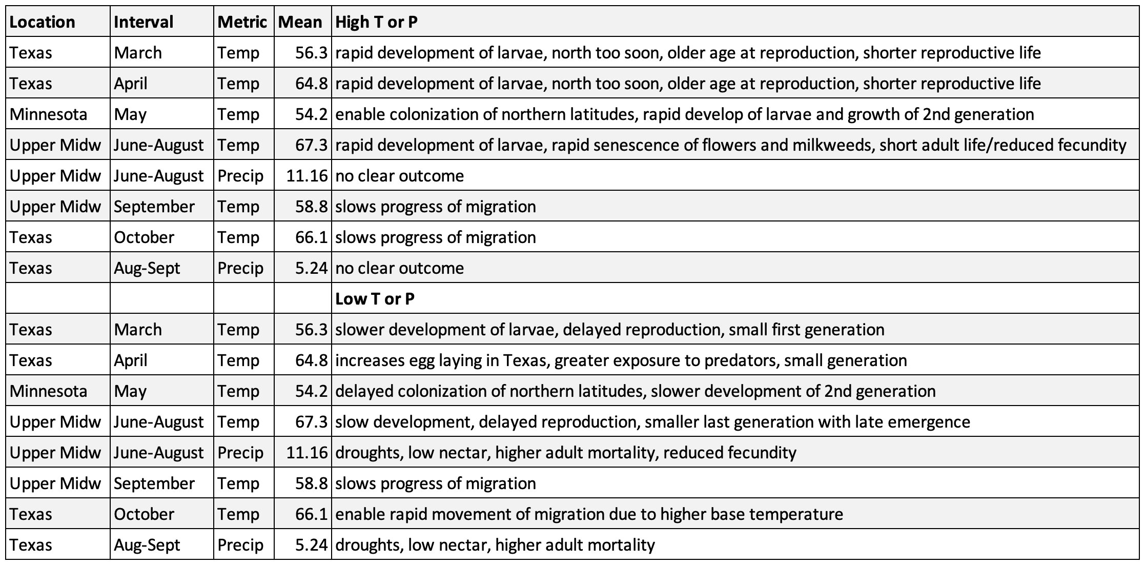
The interpretations for the effects of deviations that exceed the average condition are summarized in Table 3. Most of these interpretations reflect expected responses to extreme highs or lows for insects.

Table 3. Interpretations of deviations that substantially exceed the ranges for “average” conditions.

Results and Discussion

Two periods of contrasting outcomes are evident in Table 2. The period from 1927-1936 is characterized by a large number of unfavorable events most of which resulted in low end of season numbers. In contrast, the populations likely grew in the five years from 1937 though 1941. There were only three months in these years – all in March in Texas – with strong unfavorable measures that otherwise feature average conditions.

This record contrasts strongly with the outcomes from 1994-2022 in two ways. In that record, there was only one year in which precipitation was unfavorable in the Upper Midwest (2012, -2.27inches) while there were 7 such years in the 1927-1936 interval. Surprisingly, there were 5 years during which the March temperatures in Texas were well below the long-term averages – in contrast to none in the more recent period.

Cold temperatures in these years surely delayed the recolonization of Texas by monarchs returning from Mexico and slowed the growth of the first generation. These conditions probably limited the size of the first generation as well. In 1931, low March and April temperatures may have delayed the development of the population for an entire month or the equivalent of an entire generation. Low May temperatures in Minnesota are associated with declines in both the early and most recent records. These low temperatures delay the colonization of the summer breeding area north of 40N and the development of the second generation. During the summer months in the Upper Midwest, both low (1927) and high (1933,1936) extremes contributed to declines. High temperatures during September in the Upper Midwest may also have contributed to the declines in 1931, 1933 and 1936.

Although it is impossible to infer the number of monarchs that survived to overwinter from 1927-1941, it is likely that the numbers were quite low during the first 10 years of this period, perhaps even lower than the 0.67hectares recorded in 2013. There were 7 years from 1927-1936 with one or more deviation that exceeded any deviation seen in the last 29years. The lowest of the low points could have been at the end of 1931, the end of three consecutive years with strongly unfavorable conditions or perhaps at the end of 1936, a year with several unfavorable deviations from the long-term means.

So, while the region of the dust bowl didn’t contribute to declines in monarch numbers from 1930-1939, the conditions in those years from Texas to the central Dakotas and east to the Ohio Valley surely did. This was a remarkable interval. There is no other period in the record from 1895 to the present in which the growing season conditions were so similar from year and so damaging. And, no other period that has had such a profound impact on the people in affected areas. The lessons learned changed agriculture, land management and more. We need to remember those lessons as we draw down the Ogallala aquifer.

References

Climate at a Glance: Regional and State Time Series, published June 2023, retrieved on July 10, 2023.

Egan, Timothy (2006). The Worst Hard Time: The Untold Story of Those Who Survived the Great American Dust Bowl. Houghton Mifflin Harcourt. ISBN 978-0-618-77347-3.

Nielsen-Gammon JS, Holman A, Buley S, Jorgensen J, Escobedo C, Ott J, Dedrick J, Van Fleet A (2021) Assessment of Historic and Future Trends of Extreme Weather in Texas, 1900- 2036: 2021 Update. Document OSC-202101, Office of the State Climatologist, Texas A&M University, College Station, 44 pp.

Taylor, O.R., et. al., (in prep) Geographic and temporal variation in monarch butterfly migration success.

Figure 2. Google Earth image of dust bowl region. There are no detailed weather records for this region in the 1930s – not even for cities like Pueblo and Amarillo. As far as state records are concerned, those of Kansas are most appropriate even though about half the state is to the east of the dust bowl area.

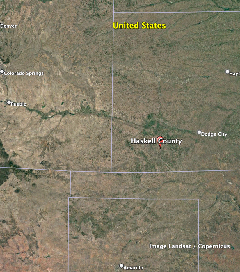
Figure 3. Part of Haskell County, KS showing center pivot irrigation.

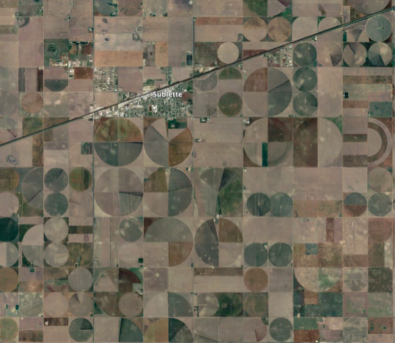
Figure 4. Region from which most monarchs originate that reach the overwintering sites in Mexico.